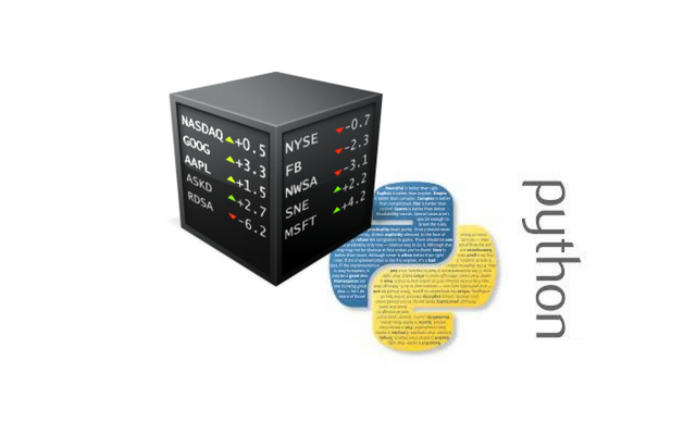
How to use Python for Algorithmic Trading on the Stock Exchange Part 1
Technologies have become an asset – financial institutions are now not only engaged in their core business but are paying much attention to new developments. We have already told you that in the world of high-frequency trade the best results are achieved by owners of not only the most efficient but also fast software and hardware.
Among the most popular programming languages:
are often used. The guide published on the DataCamp website is about how to start using Python to create financial applications – we present you with a series of articles-adaptations of the chapters of this material.
The structure of the manual:
- The first part is intended for beginners in the market, it will deal with the design of financial markets, stocks and trading strategies, time series data, and what will be needed to start the development.
- The second part introduces an introduction to working with time series data and financial analysis tools, such as calculating volatility and moving averages, using the Pandas Python library.
- Then we proceed to the immediate development of a simple impulse trading strategy.
- In the fourth part, we will talk about how to conduct backtest strategies on historical data.
- In the end, the questions of strategy optimization will be touched upon to increase its productivity, as well as to evaluate its performance and reliability.
Introduction: a simple language about the structure of the sphere of finance
Before plunging into the world of trading strategies, it makes sense to touch on the basic concepts. However, this does not mean that what will be discussed below is calculated entirely for beginners. It will be great if you first become familiar with the course on using Python to work with data, and also imagine how to work with lists and packages of Python, and also at least at a basic level are familiar with NumPy and Pandas.
Stock and trading on the exchange
- When a company wants to continue developing its business, launch new projects or expand, the shares can be used as a financing instrument. The share represents a share in the ownership of the company, shares are exchanged for money. Shares can be bought and sold: participants in such transactions conduct transactions with pre-existing shares.
- The price at which a specific share will be sold or bought can constantly change, regardless of the business indicators of the company that issued the stock: everything is determined by supply and demand. It is important to understand the difference between stocks and, for example, bonds (bonds), which are used to attract borrowed funds.
- When it comes to trading, it can be considered not only the sale and purchase of shares – the transaction can be concluded for different assets, including both financial instruments, and, for example, precious metals or resources like oil.
- When buying shares, the investor gets a certain share in the company, from which it can in the future make a financial gain by selling this stake. Strategies can differ: there are long (long) deals, concluded in the hope of further growth of the stock, and short, when the investor assumes that the shares will become cheaper, so he sells the shares in the hope of “buying back” them at a lower price in the future.
- The development of a trading strategy involves several stages, which seems, for example, to build machine learning models: first you need to formulate a strategy and describe it in a format that allows you to run it on the computer, then you need to test the performance of the resulting program, optimize it, and then evaluate the effectiveness And reliability of work.
- Trading strategies are usually checked using backtesting: this is the approach by which the strategy is “run” on historical data about trades – on their basis the program generates trades. This makes it possible to understand if such a strategy would bring an income with the development of the market situation that was observed in the past. Thus, we can preliminarily evaluate the prospects of the strategy in real-time trading. At the same time, there is no guarantee that good indicators on historical data will be repeated when working in a real market.
Time series data
The time series is a sequence of digital data obtained at consecutive equal intervals of time. In the sphere of finance, such series are used to track price movements over a certain period of time, recorded at equal intervals. Here’s how it looks:
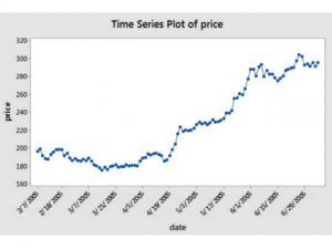
On X-axis there are dates and the price is on the Y-axis. “Consecutive equal time intervals” in this case means that the date axis is located at a two-week interval: you can compare 3/7/2005 and 3/31/2005, and also 4/5/2005 and 4/19/2005 (here the dates are recorded in the US format, when the month comes first, then the day).
- However, financial data usually does not include two parameters (price and date), but five – in addition to the value of the trading period, this is the opening price of the trading period, the highest and lowest price within it, as well as the price at the moment of closing the period. This means that if we consider the day period, the analysis of the data will give us information on the level of which the price was at the moment of start and end of trading on the selected day, and also what was the maximum and minimum price during the bidding.
Above, the basic concepts that you need to know in order to continue the study of this manual have been described.
Fundamentals of Python for Finance: Pandas
- One of the most popular tools when using Python for developing financial applications is the Pandas package. It is needed at the very beginning, but as you go deeper into the development process, you will need packages like NumPy, SciPy, and Matplotlib.
- First, we focus on Pandas and apply this tool to the analysis of time series. Below we will talk about how to import, analyze and manipulate data using this package.
Importing financial data
- The pandas-data reader package allows you to receive data from sources such as Google, Yahoo! Finance or the World Bank – more details about the available data sources are written in the documentation. This guide will consider receiving data from Yahoo! Finance. To get started, you need to install the latest version of the package using pip:
pip install pandas-datareader
Instructions for installing the version in development are presented here.
import pandas_datareader as pdr
import datetime
aapl = pdr.get_data_yahoo('AAPL',
                          start=datetime.datetime(2006, 10, 1),
                          end=datetime.datetime(2012, 1, 1))
- Not so long ago in the Yahoo API, there were changes, so to start working independently with the library you need to install fixes, which will allow waiting for the official patch. More details are described here. However, for this manual, the data was downloaded in advance, so there will be no problems with its study.
- It is also important to understand that although the pandas-data reader is a handy tool for loading data, it is by far not the only one for Python. You can also use libraries like Quandl, which allows you to retrieve data from Google Finance:
import quandl
aapl = quandl.get("WIKI/AAPL", start_date="2006-10-01", end_date="2012-01-01")
- Also, many know that in the field of finance for data analysis is very popular Excel. For the convenience of future work, you can integrate this tool with Python (for more details see the link).
Work with time series data
- To import the data, we used pandas_datareader. As a result, an all object arose-it’s a DataFrame, that is, a two-dimensional named data structure with columns of potentially different types. The first thing to do when working with such a frame is to run the head () and tail () functions in order to look at the first and last columns of the data frame. To get a useful statistical summary of the downloaded data, you can use the describe () function.
An example of this code can be found on the source material page.
- The data contains four columns with the price of opening and closing the trading period, as well as the maximum and minimum price – we consider the daily intervals and shares of Apple. Also, we get two additional columns: Volume and Adj Close. The first one is used to fix the number of shares with which transactions were made on the trading day. The second column is the adjusted closing price, which means that in the closing price of the period, all actions with shares that could have been committed before the opening of the next trading day were added.
- If you want to save data to a CSV file, you can do this using the to_csv () function, and you can read the file using read_csv () – this is useful for situations where the data source is changing and access to it is temporarily lost.
import pandas as pd
aapl.to_csv('data/aapl_ohlc.csv')
df = pd.read_csv('data/aapl_ohlc.csv', header=0, index_col='Date', parse_dates=True)
- After a basic analysis of the downloaded data, it’s time to move on. To do this, for example, you can study indexes and columns, for example, selecting the last ten rows of a particular column. This is called a subsetting since only a small set of available data is taken. The resulting subset is a series, that is, a one-dimensional named array.
- In order to look at the index and columns of data, you should use the index and columns attributes. Then you can select a subset of the last ten observations in the column. To isolate these values, use square brackets. The last value is placed in the variable ts, and its type is checked using the type () function.
# Inspect the index
aapl.index

# Inspect the columns
aapl.columns

# Select only the last 10 observations of `Close`
ts = aapl['Close'][-10:]

# Check the type of `ts`
type(ts)
- The use of square brackets is convenient, but this is not the most characteristic way of working with Pandas. Therefore, we should also consider the functions lock () and clock (): the first one is used for label-based indexing, and the latter is used for positional indexing.
- In practice, this means that you can pass a label like 2007 or 2006-11-01 to LOC (), and integers like 22 or 43 are passed to the iloc () function.
# Inspect the first rows of November-December 2006
print(aapl.loc[pd.Timestamp('2006-11-01'):pd.Timestamp('2006-12-31')].head())

# Inspect the first rows of 2007
print(aapl.loc['2007'].head())

# Inspect November 2006
print(aapl.iloc[22:43])

# Inspect the 'Open' and 'Close' values at 2006-11-01 and 2006-12-01
print(aapl.iloc[[22,43], [0, 3]])
- If you look closely at the results of the partitioning procedure, you will see that in the data are missing certain days. Further analysis of the pattern will show that usually, two or three days are not enough. These are weekends and public holidays, during which there are no exchange trades.
- In addition to indexing, there are several ways to learn about data more. You can, for example, try to create a sample of 20 lines of data, and then reformat them in such a way that appl is not a daily value and a monthly one. You can do this using the sample () and resample () functions:
# Sample 20 rows
sample = aapl.sample(20)

# Print `sample`
print(sample)

# Resample to monthly level
monthly_aapl = aapl.resample('M').mean()

# Print `monthly_aapl`
print(monthly_aapl)
- Before moving on to data visualization and financial analysis, you can begin to calculate the difference between the opening and closing prices of the trading period. This arithmetic operation can be done using Pandas – you need to subtract the values of the Open column of the appl data from the Close column. Or, in other words, subtract aapl.Close from aapl.Open. The resulting result will be stored in a new column of the aapl data frame called diff, which can be deleted using the del function:
# Add a column `diff` to `aapl`
aapl['diff'] = aapl.Open - aapl.Close

# Delete the new `diff` column
del aapl['diff']
- The resulting absolute values can already be useful in the development of a financial strategy, but usually, a deeper analysis is required, for example, the percentage of growth or decline in the price of a particular share.
Visualization of time series data
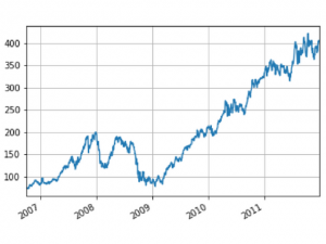
- In addition to analyzing data using the head (), tail (), and indexing, you can also render them. Thanks to the integration of Pandas with the tool for creating Matplotlib charts, this can be done quite easily. You just need to use the plot () function and pass the relevant parameters to it. In addition, if you add the grid parameter, the resulting graph will be superimposed on the grid.
# Import Matplotlib's `pyplot` module as `plt`
import matplotlib.pyplot as plt

# Plot the closing prices for `aapl`
aapl['Close'].plot(grid=True)

# Show the plot
plt.show()
This code gives this graph:
In the next part of the manual, we’ll talk about the financial analysis of time series data using Python.
To be continued
If you looking even for more features on how you can use Python such as:
- Building Interactive Python Tools with Excel as a Front-End.
- PyXLL – The Python Excel Add-In.
- Reading and Writing Excel workbooks
Then you might be interested to check this article:
