Classification Of Large Amounts Of Data On Apache Spark Using Arbitrary Machine Learning Models

Hello! Today we will talk about the classification of large amounts of data using models built using almost any available library of machine learning. In this series of two articles, we will consider the following questions.

• How to present a model of machine learning as a service (Model as a Service)?
• How are the tasks of distributed processing of large amounts of data physically performed using Apache Spark?
• What problems arise when Apache Spark interacts with external services?
  How can using the Akka-streams and Akka-HTTP libraries, as well as the
• Reactive Streams approach, effectively organize Apache Spark’s interaction with external services?

Initially, we planned to write one article, but since the amount of material was large enough, we decided to break it into two parts. Today in the first part we will consider the general statement of the problem, as well as the main problems that need to be solved in the implementation. In the second part, we’ll talk about the practical implementation of this task using the Reactive Streams approach.

We know one team of data analysts who, with a wide range of tools (such as scikit-learn, facebook fastText, xgboost, tensorFlow, etc.) are engaged in training machine learning models. De facto, the main programming language that analysts use is Python. Almost all libraries for machine learning, even originally implemented in other languages, have an interface in Python and are integrated with the main Python libraries (primarily with NumPy).

On the other hand, the Hadoop ecosystem is widely used to store and process large amounts of unstructured data. In it, the data is stored on the HDFS file system in the form of distributed replicated blocks of a certain size (usually 128 MB, but it is possible to configure). The most efficient algorithms for processing distributed data try to minimize the network interaction between cluster machines. To do this, the data must be processed on the same machines where they are stored.

• Of course, in many cases, network interaction cannot be completely avoided, but, nevertheless, one must try to perform all tasks locally and minimize the amount of data that will need to be transmitted over the network.

This principle of processing distributed data is called “move computations to data” (move computations close to data). All the main frameworks, mainly Hadoop MapReduce and Apache Spark, adhere to this principle. They determine the composition and sequence of specific operations that will need to be run on machines where the required data blocks are stored.

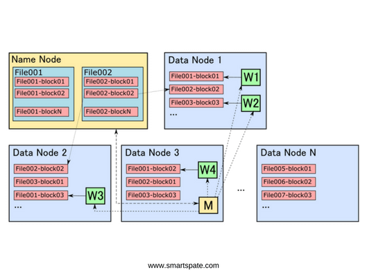
Figure 1. HDFS cluster consists of several machines, one of which is Name Node, and the rest – Data Node. The Name Node stores information about the files included in their composition of blocks, and about the machines where they are physically located. The Data Node stores the blocks themselves, which are replicated to several machines to improve reliability. Data processing tasks are also started on the Data Node. Tasks consist of the main process (Master, M), which coordinates the start of work processes (Worker, W) on machines where the necessary data blocks are stored.

• Virtually all components of the Hadoop ecosystem are run using the Java Virtual Machine (JVM) and are tightly integrated. For example, to run tasks written with Apache Spark to work with data stored on HDFS, almost no additional manipulation is required: the framework provides this functionality out of the box.

Unfortunately, most libraries intended for machine learning assume that data is stored and processed locally. At the same time, there are also libraries that are tightly integrated with the Hadoop-ecosystem, for example, Spark ML or Apache Mahout. However, they have a number of significant drawbacks. First, they provide much fewer realizations of machine learning algorithms. Secondly, not all data analysts know how to work with them. The advantages of these libraries can be attributed to the fact that they can be used to train models on large volumes of data using distributed computing.

• However, data analysts often use alternative methods to train models, in particular, libraries that enable the use of the GPU. We will not discuss the training of models in this article, because of we
  want to focus on the use of ready models built with the help of any accessible machine learning library for the classification of large amounts of data.

So, the main task that we are trying to solve here is the application of machine learning models to large amounts of data stored on HDFS. If we could use the SparkML module from the Apache Spark library, which implements the basic algorithms of machine learning, then the classification of large amounts of data would be a trivial task:

val model: LogisticRegressionModel = LogisticRegressionModel.load("/path/to/model")
val dataset = spark.read.parquet("/path/to/data")
val result = model.transform(dataset)

Unfortunately, this approach works only for algorithms implemented in the SparkML module (the full list can be found here). In the case of using other libraries, and also implemented not on the JVM, everything becomes much more complicated.

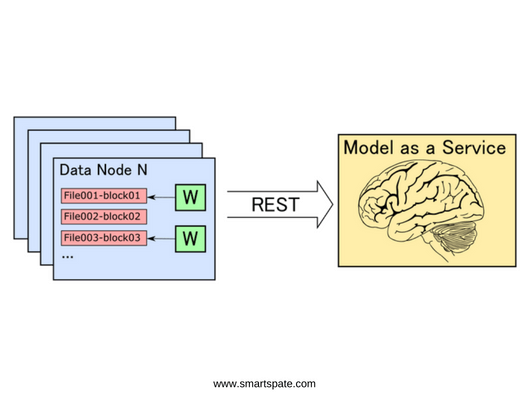
To solve this problem, we decided to wrap the model in the REST-service. Accordingly, when starting the task of classifying data stored on HDFS, it is necessary to organize the interaction between the machines on which the data is stored and the machine (or cluster of machines) on which the classification service is started.

Figure 2. The concept of Model as a Service

Description of the python classification service

In order to present the model in the form of a service, it is necessary to solve the following tasks:

• Effective access to the model via HTTP;
• Ensure the most efficient use of the resources of the machine (primarily all processor cores and memory);
• Ensure resistance to high loads;
• Provide the possibility of horizontal scaling.

Access to the model via HTTP is quite simple: for Python, a large number of libraries have been developed that allow you to implement the REST access point using a small amount of code. One of these micro-frames is Flask. The implementation of the classification service on Flask is as follows:

from flask import Flask, request, Response
model = load_model()
n_features = 100
app = Flask(__name__)

@app.route("/score", methods=['PUT'])
def score():
inp = np.frombuffer(request.data, dtype='float32').reshape(-1, n_features)
result = model.predict(inp)
return Response(result.tobytes(), mimetype='application/octet-stream')

if __name__ == "__main__":
app.run()

Here, when the service starts, we load the model into memory and then use it when calling the classification method. The load_model function loads the model from some external source, whether it’s a file system, a key-value repository, etc.

A model is an object that has a method to predict. In the case of classification, it takes on an input some feature vector of a certain size and outputs either a boolean value indicating whether the specified vector is suitable for the given model, or some value from 0 to 1, to which the cut-off threshold can then be applied: anything above the threshold, is a positive result of the classification, the rest is not.

The feature-vector that we need to classify, we pass in a binary form and deserialize it into a numpy array. It would be overhead to make an HTTP request for each vector. For example, in the case of a 100-dimensional vector and using for float32 values the complete HTTP request, including the headers, would look something like this:

PUT /score HTTP/1.1
Host: score-node-1:8099
User-Agent: curl/7.58.0
Accept: */*
Content-Type: application/binary
Content-Length: 400

[400 bytes of data]

As you can see, the efficiency of such a request is very low (400 bytes of payload / (133 bytes header + 400 bytes body) = 75%). Fortunately, in nearly all libraries, the predict method allows us to accept a vector instead of [1 x n], and, [m x n] a matrix, and, accordingly, output the result immediately for m input values.

• In addition, the numpy library is optimized for working with large matrices, allowing to effectively use all available resources of the machine. Thus, we can send one rather a large number of feature vectors in one query, deserialize them into a numpy matrix of size, [m x n], classify, and return the vector, [m x 1] from Boolean or float32 values. As a result, the efficiency of HTTP interaction when using a matrix of 1000 lines becomes almost equal to 100%. The size of HTTP headers, in this case, can be neglected.

To test the Flask service on the local machine, you can run it from the command line. However, this method is absolutely not suitable for industrial operation. The fact is that Flask is single-threaded and, if we look at the CPU load diagram while the service is running, we will see that one core is loaded by 100%, and the rest is idle. Fortunately, there are ways to use all the machine cores: for this, Flask needs to be run through the uwsgi web application server. It allows you to optimally configure the number of processes and threads so as to ensure a uniform load on all the cores of the processor. In more detail with all the options for setting up uwsgi, you can read here.

It is better to use nginx as an entry point over HTTP since uwsgi can be unstable in case of high loads. Nginx also accepts the entire incoming query flow for itself, filters out invalid queries, and doses the load on uwsgi. Nginx interacts with uwsgi via Linux sockets using a process file. An exemplary nginx configuration is shown below:

server {
listen 80;
server_name 127.0.0.1;
location / {
try_files $uri @score;
}
location @score {
include uwsgi_params;
uwsgi_pass unix:/tmp/score.sock;
}
}

As we can see, it turned out to be quite a complicated configuration for one machine. If we need to classify large amounts of data, this service will receive a high number of requests, and it can become a bottleneck. The solution to this problem is horizontal scaling.

For convenience, we pack the service into the Docker container and then deploy it to the required number of machines. If you want, you can use automated deployment tools such as Kubernetes. An example Dockerfile structure for creating a container with a service is shown below.

FROM ubuntu

#Installing required ubuntu and python modules
RUN apt-get update
RUN apt-get -y install python3 python3-pip nginx
RUN update-alternatives --install /usr/bin/python python /usr/bin/python3 1
RUN update-alternatives --install /usr/bin/pip pip /usr/bin/pip3 1
RUN pip install uwsgi flask scipy scikit-learn

#copying script files
WORKDIR /etc/score
COPY score.py .
COPY score.ini .
COPY start.sh .
RUN chmod +x start.sh

RUN rm /etc/nginx/sites-enabled/default
COPY score.nginx /etc/nginx/sites-enabled/

EXPOSE 80

ENTRYPOINT ["./start.sh"]

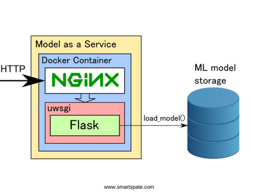
Figure 3. Service scheme for classification

A brief description of Apache Spark in the Hadoop ecosystem

Now consider the process of processing data stored on HDFS. As we have already noted, the principle of transferring computations to data is used for this. To run the processing tasks, you need to know which machines store the data blocks we need to run the processes involved in the processing directly on them. It is also necessary to coordinate the launch of these processes, restart them in case of abnormal situations, if necessary, aggregate the results of performing various subtasks, etc.

All these tasks are solved by a number of frameworks working with the Hadoop ecosystem. One of the most popular and convenient is Apache Spark. The main concept around which the entire framework is built is RDD (Resilient Distributed Dataset). In general, RDD can be viewed as a distributed collection that is resistant to falls. RDD can be obtained in two main ways:

1. Creation from an external source, such as a collection in memory, a file or directory on the file system, etc .;
2. A transformation from another RDD by applying transformation operations. RDD supports all the basic operations for working with collections, such as map, flatMap, filter, group, join, etc.

It is important to understand that RDD, unlike collections, is not the data itself, but the sequence of operations that must be performed on the data. Therefore, when you call the transformation operations, no work actually takes place, and we just get a new RDD, which will contain one operation more than the previous one. The very same work is started when calling the so-called terminal operations, or actions. These include saving to a file, saving to a collection in memory, counting the number of items, etc.

When the terminal operation is started, Spark builds an acyclic operations graph (DAG, Directed Acyclic Graph) on the basis of the resulting RDD and sequentially runs them on the cluster according to the received graph. When building a DAG based on RDD, Spark performs a number of optimizations, for example, if possible, combines several successive transformations into a single operation.

RDD was the primary unit of interaction with the Spark API in versions of Spark 1.x. In Spark 2.x, the developers said that now the main concept for interaction is Dataset. Dataset is an add-on over RDD with support for SQL-like interaction. When using Dataset API Spark allows you to use a wide range of optimizations, including low-level ones. But in general, the basic principles applicable to RDD are also applicable to Dataset.

• More details about the work of Spark can be found in the documentation on the official website.

Consider an example of the simplest classification on Spark without using external services. There is a fairly meaningless algorithm implemented here that considers the proportion of each of the Latin letters in the text, and then counts the standard deviation. Here, in the first place, it is important to pay attention to the basic steps used when working with Spark.

case class Data(id: String, text: String)
case class Features(id: String, vector: Array[Float])
case class Score(id: String, score: Float) //(1)

def std(vector: Array[Float]): Float = ??? //(2)

val ds: Dataset[Data] = spark.read.parquet("/path/to/data").as[Data] //(3)

val result: Dataset[Score] = ds.map {d: Data => //(4)
val filteredText = data.text.toLowerCase.filter { letter =>
'a' <= letter && letter <= 'z'
}
val featureVector = new Array[Float](26)
val aLetter = 'a'
if (filteredText.nonEmpty) {
filteredText.foreach(letter => featureVector(letter) += 1)
featureVector.indicies.foreach { i =>
featureVector(i) = featureVector(i) / filteredText.length()
}
}
Features(d.id, featureVector)
}.map {f: Features =>
Score(f.id, std(f.vector)) //(5)
}

result.write.parquet("/path/to/result") //(6)

In this example:

• We define the structure of input, intermediate and output data (we define input as a certain text with which a certain identifier is associated, intermediate data associate an identifier with a feature vector, and output matches an identifier with some numeric value);
• Define the function for calculating the resultant value by the feature-vector (for example, standard deviation, the implementation is not shown);
• Define the original Dataset as data stored on HDFS in parquet format along with the path/path/to/data;
• Define the intermediate Dataset as an element-wise transformation (map) from the original Dataset;
• Similarly, we define the resultant Dataset through the elementwise transformation from the intermediate;
• Save the resulting Dataset to HDFS in parquet format along with the path/path/ to/result. Since saving to a file is a terminal operation, the calculations themselves are started at this stage.

Apache Spark works as a master-worker. When the application starts, the main process, called the driver, starts. It executes the code responsible for the formation of RDD, on the basis of which the calculations will be performed.

When the terminal operation is called, the driver generates a DAG based on the resulting RDD. The driver then initiates the launch of workflows, called executors, in which the data will be processed directly. After running the workflows, the driver passes them the executable that needs to be executed and also indicates to which part of the data it needs to be applied.

Below is the code for our example, in which sections of code executed on the executor are highlighted (between the lines of the executor part begin and executor part end). The rest of the code is executed on the driver.

case class Data(id: String, text: String)
case class Features(id: String, vector: Array[Float])
case class Score(id: String, score: Float)

def std(vector: Array[Float]): Float = ???

val ds: Dataset[Data] = spark.read.parquet("/path/to/data").as[Data]

val result: Dataset[Score] = ds.map {
// --------------- EXECUTOR PART BEGIN -----------------------
d: Data =>
val filteredText = data.text.toLowerCase.filter { letter =>
'a' <= letter && letter <= 'z'
}
val featureVector = new Array[Float](26)
val aLetter = 'a'
if (filteredText.nonEmpty) {
filteredText.foreach(letter => featureVector(letter) += 1)
featureVector.indicies.foreach { i =>
featureVector(i) = featureVector(i) / filteredText.length()
}
}
Features(d.id, featureVector)
// --------------- EXECUTOR PART END -----------------------
}.map {
// --------------- EXECUTOR PART BEGIN -----------------------
f: Features => Score(f.id, std(f.vector))
// --------------- EXECUTOR PART END -----------------------
}

result.write.parquet(“/path/to/result”)

In the Hadoop ecosystem, all applications are started in containers. A container is a certain process running on one of the cluster machines, to which a certain number of resources are allocated. The launch of the containers is handled by the YARN resource manager. It determines to which of the machines there is a sufficient number of cores of the processor and RAM, and also whether the necessary data blocks for processing are available on it.

When you run the Spark application, YARN creates and runs a container on one of the cluster machines in which it starts the driver. Then, when the driver prepares the DAG for operations that need to be run on the executables, YARN starts additional containers on the appropriate machines.

• As a rule, it is enough for the driver to allocate one core and a small amount of memory (if, of course, then the result of calculations will not be aggregated on the driver in memory). For executors, in order to optimize resources and reduce the total number of processes in the system, you can select more than one core: in this case, the performer will be able to perform several tasks simultaneously.

But here it is important to understand that in the event of a drop in one of the tasks running in the container or in case of a lack of resources, YARN may decide to stop the container, and then all tasks that were performed in it must be restarted on another performer. In addition, if we allocate a sufficiently large number of cores per container, then there is a possibility that YARN will not be able to start it. For example, if we have two machines with two cores left unused, we can run each on a container that requires two cores, but we can not run one container that requires four cores.

Now let’s see how the code from our example will be executed directly on the cluster. Imagine that the size of the raw data is 2 terabytes. Accordingly, if the block size on HDFS is 128 MB, then there will be 16,384 blocks. Each block is replicated to several machines to ensure reliability. For simplicity, let’s take the replication factor equal to two, that is, there will be only 32768 available blocks. Suppose that for storage we use a cluster of 16 machines. Accordingly, on each of the machines in the case of uniform distribution will be approximately 2048 blocks or 256 gigabytes per machine. On each of the machines, we have 8 processor cores and 64 gigabytes of RAM.

For our task, the driver does not need a lot of resources, so we’ll allocate 1 core and 1 GB of memory for it. The performers will be given 2 cores and 4 GB of memory. Suppose that we want to maximize the use of cluster resources. Thus, we get 64 containers: one for the driver, and 63 – for the performers.

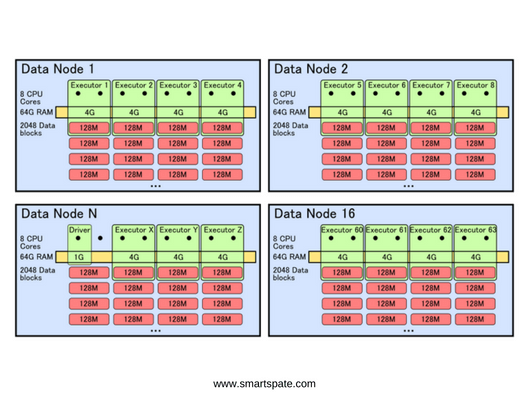
Figure 4. The processes running on the Data Node and the resources they use.

Since in our case we only use map operations, our DAG will consist of one operation. It consists of the following:

• Take one block of data from the local hard drive,
• Convert data,
• Save the result to a new block on your local disk.

In total, we need to process 16384 blocks, so each performer must perform 16384 / (63 executors * 2 cores) = 130 operations.

Thus, the lifecycle of the executor as a separate process (in the event that everything happens without a fall) will look like this.

• Start the container.
• Obtaining a task from the driver in which the block ID and the required operation will be. Since we have allocated two cores to the container, the performer receives two tasks at once.
• Execute the task and send the result to the driver.
• Getting the next task from the driver and repeating steps 2 and 3 until all the blocks for this local machine are processed.
• Stop the container.

Note: more complex DAGs are obtained if you need to redistribute intermediate data between machines, usually for grouping operations (groupBy, reduceByKey, etc.) and joins that are beyond the scope of this article.

The main problems of Apache Spark interaction with external services

In the event that we need to access some external service within the map operation, the task becomes less trivial. Suppose that for interaction with an external service there is an object of the ExternalServiceClient class. In general, before starting work, we need to initialize it, and then call it as needed:

val client = ExternalServiceClient.create () // Initialize
val score = client.score (featureVector) // Call the service.

Typically, the initialization of the client takes some time, so, as a rule, it is initialized at application startup, and then used to receive a client instance from some global context, or a pool. Therefore, when a container with Spark executor gets a task that requires interaction with an external service, it would be nice to get an initialized client before starting work on the data set, and then re-use it for each element.

In Spark, you can do this in two ways. First, if the client is serializable (the client itself and all its fields should expand the interface java.io.Serializable), then it can be initialized on the driver and then transferred to the executors via the mechanism of broadcast variables.

val client = ExternalServiceClient.create()
val clientBroadcast = sparkContext.broadcast(client)
ds.map { f: Features =>
val score = clientBroadcast.value.score(f.vector)
Score(f.id, score)
}

In case the client is not serializable, or the client initialization is a process that depends on the settings of the particular machine on which it is started (for example, for balancing, requests from one part of the machines should go to the first server machine, and for the second one to the second one) then the client can be initialized directly on the performer.

To this end, RDD (and Dataset) has a mapPartitions operation, which is a generalized version of the map operation (if you look at the source code of the RDD class, then the map operation is implemented via mapPartitions). The function passed to the mapPartitions operation is run once for each block. The input of this function is an iterator for the data that we will read from the block, and at the output, it should return an iterator for the output data corresponding to the input block:

ds.mapPartitions {fi: Iterator[Features] =>
val client = ExternalServiceClient.create()
fi.map { f: Features =>
val score = client.score(f.vector)
Score(f.id, score)
}
}

In this code, a client to an external service is created for each block of raw data. This, of course, is better than creating a client each time to process each element, and in many cases, this is a very acceptable solution. However, a little further on I’ll show you how you can create an object that will be initialized once at the start of the container and then used to start all the tasks that come to this container.

The operation of processing the resulting iterator is single-threaded. Let me remind you that the main pattern of access to the structure of the iterator type is a sequential call to hasNext and next methods:

while (i.hasNext()) {
val item = i.next()
…
}

If we have two kernels allocated for the artist, then they will have only two main workflows that process the data. Let me remind you that if we have 8 cores on the machine, then YARN will not allow it to run more than 4 executor processes with 2 cores, respectively, we will have only 8 threads per machine. For local calculations, this is the optimal choice, since this will ensure maximum utilization of computing power with minimal overhead for flow control. However, in the case of interaction with external services, the picture changes.

• When using external services, productivity is one of the most important issues. The simplest way of implementation is to use the asynchronous client, in which we address the service for each element, and, having received a response from it, we form the resulting value. However, this approach has one significant drawback: for synchronous interaction, a thread synchronously calling an external service is blocked for the time of interaction with this service.

The fact is that when we call the hasNext method, we expect to get an unambiguous answer to the question whether there are any other elements for processing. In case of uncertainty (for example, when we sent a request for an external service and do not know if it will return an empty or non-empty answer), we have nothing else to do but wait for a response, thus blocking the thread that caused this method. Therefore, the iterator is a blocking data structure.

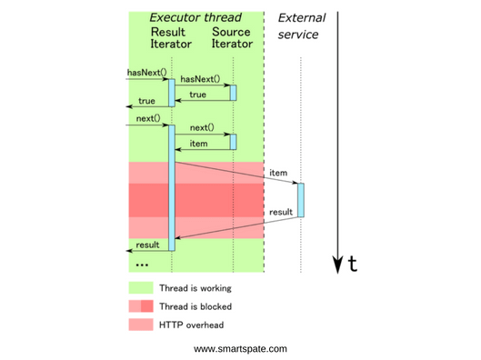
Figure 5. Element-by-element processing of the iterator, obtained as a result of calling a function passed to mapPartitions, occurs in one thread. As a consequence, we get extremely inefficient use of resources.

As you remember, we optimized our classification service in such a way that it allows us to process several requests simultaneously. Accordingly, we need to collect the necessary number of requests from the source iterator, send them to the service, get an answer and give them to the resulting iterator.

Figure 6. Synchronous interaction when sending a classification request for a group of elements

In fact, in this case, the performance will not be much better, because, firstly, we have to keep the main thread in the locked state while there is interaction with the external service, and, secondly, the external service is idle while we work with the result.

The final formulation of the problem

Thus, when using an external service, we must solve the problem of synchronous access. Ideally, it would be convenient to take the interaction with external services into a separate thread pool. In this case, requests to external services would be executed simultaneously with processing the results of previous requests, and thus it would be possible to use the machine resources more efficiently. For interworking between threads, a blocking queue could be used, which would serve as a communication buffer. Threads responsible for interacting with external services would put the data in the queue, and the thread handling the resulting iterator, respectively, would take them from there.

However, such asynchronous processing involves a number of additional problems.

• In case the processing speed of the resulting iterator is lower than the speed of receiving responses from external services, the buffer size will grow and buffer overflow may occur.
• In the event that an error occurred during the processing of one of the requests to external services, appropriate measures must be taken. With synchronous processing, all interaction occurs within the same thread, so it’s enough to just throw an exception. In asynchronous processing, you will need to pass the exception information from the secondary threads to the main thread and, if necessary, stop both the data reading from the source iterator and the output of the data in the resulting iterator.
• In order for the hasNext method to return false in the resulting iterator, it is necessary to make sure that all requests were answered and to signal that there will be more data in the buffer. In synchronous processing, this is quite simple: if after processing the next response the original iterator returned hasNext = false, then, accordingly, there will be no more elements. In the case of asynchronous processing, especially if we send several requests at the same time, we also need to coordinate the response, and only after receiving the last answer send a signal about the completion of processing.

About how we managed to effectively solve these problems, we will discuss in the next part. Stay Tuned!